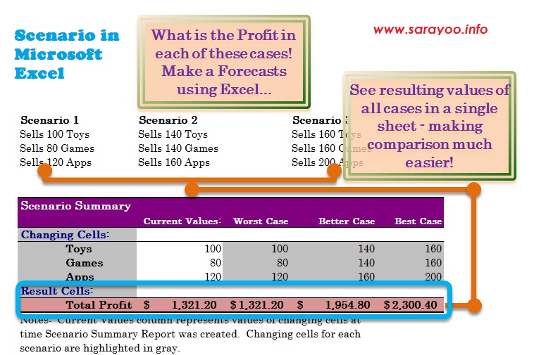
There may be times when we need to experiment with several different values in an Excel Spreadsheet to make predictions and forecasts. For example, you are selling various products. Assume that you have a profit target to meet and you want to see how much profit you will make if you sell x number of each product. You can do this in an Excel Spreadsheet easily by making use of Scenarios in the What-If-Analysis tool.
By using Scenarios, you are able to enter a set of different values in a spreadsheet, and Excel will automatically calculate the resulting values.
What is a Scenario in Excel and When to Use it?
Scenarios in Microsoft Excel allows you to enter multiple groups of variables which is substituted by Excel to produce the resulting cell values. In the following example, we want to see how much profit you will make if you are able to sell 100 Toys, 80 Games and 120 Apps. We also want to see, how much profit can be made if we are able to sell 140 Toys, 140 Games and 160 Apps or 160 Toys, 160 Games and 200 Apps, etc. These set of values (100 Toys, 80 Games, 120 Apps, etc.) can be saved as different scenarios in Excel.
In other words, scenarios in Excel helps you save and manipulate many different groups of values to change the end result and make comparisons.
You may also want to check out how to create conditional formatting in Excel and how to switch data from columns to rows and rows to column easily.
How to Create Scenarios in MS Excel?
You can create scenarios in your spreadsheet by following the steps below:
Step 1:
Open your spreadsheet. Decide which cells or values in the spreadsheet that you want to change and where the results should appear. In our example, the changing cells will be C4, D4 & E4 and the resulting cells will be: C10, D10, E10 – Profit per product and D13 showing Total Profit.
Step 2:
Click on Data tab | What-If-Analysis under Data Tools group | Scenario Manager

Step 3:

In Scenario Manager window, click Add | Fill in the scenario name, in the example here, the name is “Worst Case” for the first scenario, “Better Case” for the second one and “Best Case” for the last one. Then Click in the “Changing cells” field and select the cells where the values will be changing. In this case, these cells are: C4 to E4 (C4:E4).
Step 4:
Enter scenario values: Here you can enter your scenario value. In our example, C4 = 100, D4 = 80 and E4 = 120. And click OK.

Step 5:
Continue Step 3 and Step 4 and complete other scenarios. In our example, these will be “Better Case” (Values: 140 Toys, 140 Games and 160 Apps) and “Best Case” (Values: 160 Toys, 160 Games and 200 Apps) and fill in each case values.
How to View Each Scenario Results
Once all scenarios are entered, you can view the result by clicking on each scenarios. To do that:
Step 1:
Click on Data tab | What-If-Analysis under Data Tools group | Scenario Manager
Step 2:
Select the scenario you want to see the result of, and click Show. Adjust the scenario manager window accordingly so that you can view the resulting cells.
How to Generate a Report of all Scenarios: Scenario Summary
Clicking through each scenario and looking at the result can be difficult, especially when you want to compare the results of each scenario. To make this easier, Microsoft Excel allows us to create a Scenario Summary Report, comprising all the scenarios and results in a single report.
To create a Scenario Summary:
Step 1:
Click on Data tab | What-If-Analysis under Data Tools group | Scenario Manager
Step 2:
Click on Summary | Select Scenario summary and select the Result cell(s) and click Ok.


This will create a Scenario Summary report in a new sheet. You can edit the cell labels in the Scenario Summary to make it more readable.
Here is a video showing you how to create scenario and create summary reports.
